The Traffic Accident Reconstruction Origin -Article-


The Traffic Accident Reconstruction Origin -Article-
|

|
Statistics- A Method to Quantify Uncertainty
By Dr Oren Masory and Bill Wright Introduction The value of a drag factor, the length of a skid mark and the weight of a vehicle
are used routinely in the field of accident reconstruction. Regardless of the accuracy of
the measuring instrument none of these values will ever be exact. This "inexactness" is
called uncertainty. For example, if we determine the drag factor to be .73 is the uncertainty
Each time we use a number we should have some idea of just how that number is related to
the true quantity. This discussion will demonstrate how statistics can guide us to a method
for quantifying uncertainty. Uncertainty, an Example Problem Suppose we wish to test for the drag factor of a surface with a drag sled. It will be
used in the usual way. It will be weighed with a scale. Say the hypothetical drag sled weighs
50 Units (Note: metric readers can think kg each place the word Unit appears in this article,
English readers can think pounds). We will use the drag sled as follows. 1) It will be dragged it at constant speed on the surface in question. 2) As it is pulled at a constant speed the scale will be read to determine
the force required to pull the sled. 3) Once these two measurements are made the results will be used to find the drag
factor by dividing the force required to pull the sled by its weight. The variable that we will concern ourselves in this example is the force reading
on the scale as the sled is pulled horizontally. Let's suppose that officer A
makes ten test pulls of the sled. This set of 10 tests is called a sample. Here
are results of his tests- 25, 23, 22, 24, 25, 28, 27, 26, 26, 24 (all Units). We follow drag sled test convention and find the average of his tests. To do this we
simply add the results of each test, then divide by the number of tests. In this case the
sum is 250. 250/10 yields an average, or mean value for force of 25 Units. This
process of finding a mean is a statistical operation. The field of statistics
carries its own notation. For example, finding the average of a sample is expressed as: ![]() 0.005,
0.005,
![]() 0.05
or
0.05
or ![]() 0.5. This is an important thing to know.
0.5. This is an important thing to know.
 (1)
(1)
The reader that is unfamiliar or rusty with this notation is invited to read a short review of statistical notation .
Next a rookie investigator (officer B) wishes to try the device. He returns to the same surface and also makes ten pulls. His results are 17,19,20,21, 22,28,29,30, 31 and 33 units. By equation 1 above the average of his tests is also 25 Units.
The readings for each test in both officers sample's are presented below (Note: for the sake of illustrating a point the test results are presented in increasing force order [lowest to highest] rather than test order [test1, test 2, test 3…]).
|
Drag Sled Tests |
||||||||||
|
Officer A |
22.0 |
23.0 |
24.0 |
24.0 |
25.0 |
25.0 |
26.0 |
26.0 |
27.0 |
28.0 |
|
Officer B |
17.0 |
19.0 |
20.0 |
21.0 |
22.0 |
28.0 |
29.0 |
30.0 |
31.0 |
33.0 |
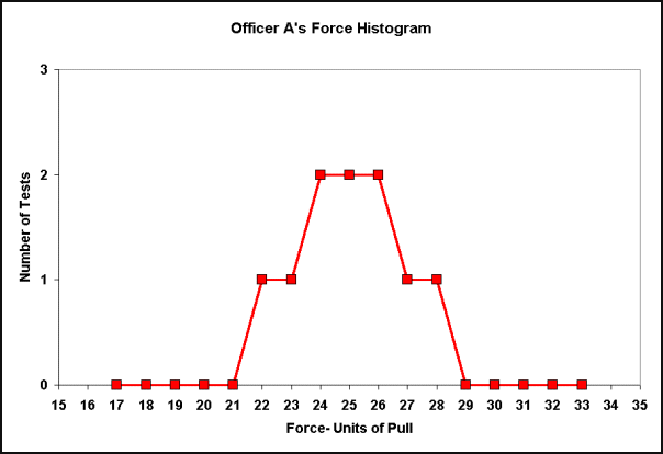
Even though both these samples have the same average or mean there is something different about them. Officer A's tests are tightly grouped about the average value of 25 lbs. Officer B's tests are much more widely varied. We can view officer A's test values graphically in a chart -Figure 1 below.

Figure 1
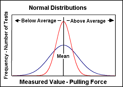
This type of chart is called a histogram. A histogram is a graphic way to see how often (the frequency) something occurs. In this case we can see from the red histogram that 6 tests had duplicate results, 24, 25, and 26 Units (2 each). Four test values occurred only once 22, 23, 27 and 28. Many other values were never observed in any test (15,16,17,18,19,20,21 and 30, 31, 32, 33, 34 (or 1145 for that matter)). Something else is apparent from looking at the chart. We can see that the values of these tests are centered about our calculated mean of 25 Units of force. Stated another way, all of officer A's tests are exactly at, or close to our average value. This type of distribution of tests is called a Normal Distribution. Another picture of a normal distribution will assist in understanding this idea.

Graphed left are two hypothetical normal distribution histograms. The scale along the bottom of the chart is associated with the actual measured value. We could think about it as the scale reading of force in the drag sled problem. The vertical axis represents the number of times (again frequency) a particular reading occurred.
Normal distributions describe a surprising number of naturally occurring events. Of most interest to the reader of this paper is the description of precision errors in measurement- in this case the ability of the scale to measure the force to pull a moving drag sled. All curves of this type have a central tendency about the mean value. They are also symmetric. That is they look similarly to the left and right of the mean value. The relative width of the curve can be described by a term called standard deviation. Standard deviation is an expression that describes how much the data varies. Variance is another statistical term. Variance is equal to the standard deviation squared. So we can see variance and standard deviation are related. The reader can get a feel for standard deviation (or variance) by comparing the red and blue lines in the figure above. It should be easy to see that the dark blue sample has a greater standard deviation (and variance) than the red one. If given the choice of these two curves as data from the drag sled pulling measurement we would choose our data to be tightly grouped, like the red curve.
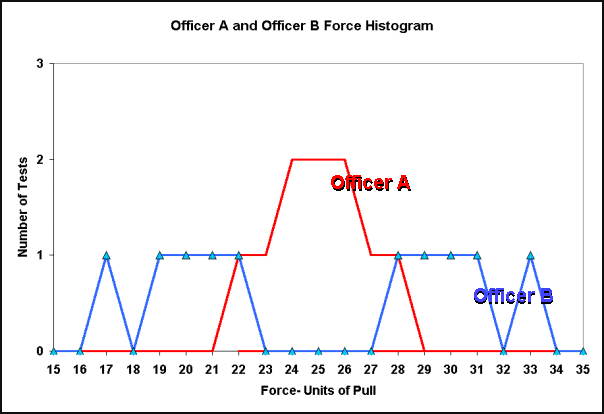
Now armed with these statistical tools to treat data we will look at the histogram of both officers' tests.

Figure 2
Viewing this histogram it should be clear from Figure 2 that officer B's sample has a greater standard deviation than officer A's. Standard deviation is central to determining uncertainty in measurement. So, in order to determine uncertainty we must first be able to calculate standard deviation.
Calculating Standard Deviation
Standard deviation is defined as
 (2)
(2)
Again the reader is offered
more detail on interpreting this notation and two options for calculating standard deviation.From Equation 2 we calculate the standard deviation of both officers' samples. By any method available the standard deviation is 1.8 Units for the experienced officer and 5.8 Units for the rookie officer. What remains is to relate both samples of 10 tests to samples that have many tests. We need one more concept to complete the procedure for finding uncertainty.
Finite and Infinite Samples
Suppose we could take an infinite number of force readings on the surface in
question. As our sample became larger and larger we would have a better and better
idea of the true value of force. The concept here is that the more tests that are
performed the better our answer and the smaller the uncertainty. This should be
intuitive to the reader- pulling the sled 10 times gives better results than pulling it
once. Similarly pulling 30 times gives better results than pulling 10 times. Ideally we
should pull an infinite number of times and have a very finely honed answer. Unfortunately
pulling a drag sled an infinite number of times takes a very long time. So instead we
choose to use a probability factor that can relate our finite number of tests to a
hypothetical infinitely large sample. This factor called a t-estimator is
taken from a table (a student-t distribution). A t-estimator relates the size of the
test sample with a sample of infinite size. From the table we choose a value,
![]() where n is the number of samples and P is the
percent of probability of the desired result.
where n is the number of samples and P is the
percent of probability of the desired result.
We now have all the necessary values to calculate uncertainty.
Uncertainty, (3)
(3)
Where,
![]() =
Our answer for uncertainty- the range in which the actual value of x lies at the given
probability.
=
Our answer for uncertainty- the range in which the actual value of x lies at the given
probability.
![]() =
The average (mean) of the tests
=
The average (mean) of the tests
![]() =
The standard deviation of the tests
=
The standard deviation of the tests
![]() =
The Number of tests in the sample
=
The Number of tests in the sample
![]() =
The t estimator from the
table
with n
samples at P probability
=
The t estimator from the
table
with n
samples at P probability
Calculating Uncertainty- Example Problems
Example 1) Suppose we wish to calculate the uncertainty in officer A's drag sled sample from above.
We will use Equation 3 from above:
 (3)
(3)
Where,
![]() = Our
answer for uncertainty- the range in which the actual value of x lies at the given
probability
= Our
answer for uncertainty- the range in which the actual value of x lies at the given
probability
![]() =
25 Units =The average (mean) of the tests calculated earlier.
=
25 Units =The average (mean) of the tests calculated earlier.
![]() =
1.8 Units = The standard deviation of officer A's tests calculated earlier.
=
1.8 Units = The standard deviation of officer A's tests calculated earlier.
![]() = 10 =
The Number of tests in the sample.
= 10 =
The Number of tests in the sample.
![]() = 2.26 =
The t estimator from the
table with n
=10 samples and P
= 95% probability.
= 2.26 =
The t estimator from the
table with n
=10 samples and P
= 95% probability.
Substituting into Equation 3 we find that

Example 2) Let's examine officer's B's tests at a confidence level of 95%. In this case,
![]() =25 Units,
=25 Units,
![]() =5.8 Units,
=5.8 Units,
![]() =10, and
=10, and
![]() = 2.26.
= 2.26.
Substituting into Equation 3

Solution: There is a 95% probability that the true force lies between 20.85 Units and 29.15 Units. These values calculate to the drag factors .42 and .58 respectively (again assuming 0 uncertainty in weight). Comparing the results of example 1 and 2 should point out potential problems in ignoring the distribution of data and simply averaging a number of tests to determine the true value for force.
Example 3) A hypothetical Electronic Measuring Device in a total station takes 5 distance measurements in rapid succession. Find the 99% confidence level for the true value of the distance measurement.
Distance Data
|
Distance 1 |
Distance 2 |
Distance 3 |
Distance 4 |
Distance 5 |
|
173.500002 |
173.500010 |
173.499998 |
173.500008 |
173.500004 |
Analysis
Certain types of measures have very small uncertainty. As we can see from Equation
3 above these are numbers where ![]() - the standard
deviation is small,
- the standard
deviation is small, ![]() - the t estimator is small,
or
- the t estimator is small,
or ![]() - the number of samples is large.
- the number of samples is large.
Examples of these small uncertainty circumstances include:
1) The total station example from above (![]() is
small).
is
small).
2) The length of a well defined skid mark. (![]() is small).
is small).
3) An accelerometer that gathers acceleration data at 100 samples per second
(![]() - is large).
- is large).
4) A measurement where the desired probability is low
(![]() - is small)
- is small)
Situations where uncertainty is great occur when these variables take opposite extremes. For example:
1) An poorly conducted sample of drag sled tests, like officer B's above-
(![]() is large).
is large).
2) A skid test with a sample of only one test-
(![]() is small and
is small and
![]() is unknown).
is unknown).
3) A distance taken with a distance-measuring wheel over irregular terrain-
(![]() is large).
is large).
4) A measurement where probability is high
(![]() - is large)
- is large)
Conclusion
Uncertainty is a fact of life for anyone that wishes to know anything quantifiable about anything. Recognizing this fact it is always smart to address the uncertainty of any number encountered. For example when presented with a speed estimate is it a minimum (where the uncertainty always exceeds the stated speed)? If not then what is the uncertainty?
In order to quantify uncertainty in any measured quantity, repetitive measurements must be taken. This is the price that must be paid in order to establish reliable and accurate measurement.
At this point the reader should feel comfortable in calculating uncertainty given a sample of measures. Once calculated the reader may be struck with the question What to do I do with the results? To answer this question, the reader is referred to a TARO paper entitled Sensitivity to Uncertainty .
Dr. Oren Masory is a Professor and the Director Robotics Center of the Mechanical Engineering Department at Florida Atlantic University in Boca Raton, FL. He can be reached at (561) 297-2693 or via Email at masoryo@fau.edu
Bill Wright is an accident investigator with the Palm Beach County Sheriffs Office in West Palm Beach, Fl (USA). He teaches accident investigation and driver training topics. He can be reached at bwright@tarorigin.com
|
Copyright ©
|